3. Robust algorithms for Regression, Classification and Clustering

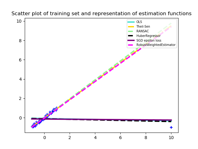
Robust statistics are mostly about how to deal with data corrupted with outliers (i.e. abnormal data, unique data in some sense). The aim is to modify classical methods in order to deal with outliers while loosing as little as possible in efficiency compared to classical (non-robust) methods applied to non-corrupted datasets. In particular, in machine learning, we want to bound the influence that any minority of the dataset can have on the prediction, see the figure for an example in regression.

3.1. What is an outlier ?

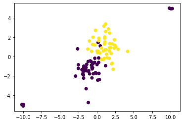
The term “outlier” refers to a discordant minority of the dataset. It is generally assumed to be a set of points situated outside the bulk of the data but there exist more complex cases as illustrated in the figure below.

Formally, we define outliers for a given task by considering points for which the loss function takes unusually high values. In the case of classification, one can consider that in the following scatter plot the points in the up-right corner are outliers while the points in the bottom-left corner are not.

Outliers can be caused by a lot of things, among them are human errors, captor errors or inherent causes. These are often found for example in biology, econometrics or datasets that describe some human relationships.

Here, we limit ourselves to linear estimators, but non-linear estimators are also plagued with the same non-robustness properties. See scikit-learn RANSAC documentation (scikit-learn) for an example of outliers for non-linear estimators.

3.2. Robust estimation with robust weighting

A lot of learning algorithms are based on a paradigm known as empirical risk minimization (ERM) which consists in finding the estimator \(\widehat{f}\) that minimizes an estimation of the risk.

\[\widehat{f} = \text{argmin}_{f\in F}\frac{1}{n}\sum_{i=1}^n\ell(f(X_i),y_i),\]

where the \(\ell\) is a loss function (e.g. the squared distance in regression problems). Said in another way, we are trying to minimize an estimation of the expected risk and this estimation corresponds to an empirical mean. However, it is well known that the empirical mean is not robust to extreme data and these extreme values will have a big influence on the estimation of \(\widehat{f}\). The principle behind the robust weighting algorithm is to rely on a robust estimator (such as median-of-means (MOM) or Huber estimator) in place of the empirical mean in the equation above [1].

In practice, one can define weights \(w_i\) that depends on the \(i^{th}\) sample, with the weight \(w_i\) being very small when the \(i^{th}\) data is an outlier and large otherwise. This way, the problem is reduced to the following optimization :

\[\min_{f}\, \frac{1}{n} \sum_{i=1}^n w_i\ell(f(X_i),y_i)\]

Remark that the weights \(w_i\) depends on \(\widehat{f}\), and the resulting algorithm is then an alternate optimization scheme, iteratively doing one step to optimize with respect to \(f\) while the weights stay fixed and then one step to estimate the weights while \(f\) stays fixed. These two steps are then repeated until convergence.

3.3. Robust estimation in practice

3.3.1. The algorithm

The approach is implemented as a meta algorithm that takes as input a base estimator (e.g., SGDClassifier, SGDRegressor or MiniBatchKMeans).

At each step, the algorithm estimates sample weights that are meant to be small for outliers and large for inliers and then we do one optimization step using the base_estimator optimization algorithm.

There are two weighting scheme supported in this algorithm: Huber-like weights and median-of-means weights. These two types of weights both come with a parameter that will determine the robustness/efficiency trade-off of the estimation.

• Huber weights : the parameter “c” is a positive real number. For small values of c the estimator is more robust but less efficient than it is for large values of c. A good heuristic consists in choosing c as an estimate of the standard deviation of the losses of the inliers. In practice, if c=None, it is estimated with the inter-quartile range.

• Median-of-means weights : the parameter “k” is a non-negative integer, when k=0 the estimator is exactly the same as base_estimator and when k=sample_size/2 the estimator is very robust but less efficient on inliers. A good heuristic consists in choosing k as an estimate of the number of outliers. In practice, if k=None, it is estimated using the number of points distant from the median of more than a 1.45 times the inter-quartile range.

  Robustness/Efficiency tradeoff and choice of parameters

  weighting	Robustness parameter	Small parameter	Large parameter
  mom	k	Non robust	Robust
  huber	c	Robust	Non robust

The choice of the optimization parameters max_iter and eta_0 are also very important for the efficiency of this estimator. It is recommended to use cross-validation to fix these hyper-parameters. Choosing eta0 too large can have the effect of making the estimator non-robust. One should also take care that it can be important to rescale the data (the same way as it is important to do it for SGD). In the context of a corrupted dataset, please use RobustScaler.

This algorithm has been studied in the context of “mom” weights in the article [1], the context of “huber” weights has been mentioned in [2]. Both weighting schemes can be seen as special cases of the algorithm in [3].

3.3.2. Comparison with other robust estimators

There are already some robust algorithms in scikit-learn but one major difference is that robust algorithms in scikit-learn are primarily meant for Regression, see robustness in regression. Hence, we will not talk about classification algorithms in this comparison.

As such we only compare ourselves to TheilSenRegressor and RANSACRegressor as they both deal with outliers in X and in Y and are closer to RobustWeightedRegressor.

Warning: Huber weights used in our algorithm should not be confused with HuberRegressor or other regression with “robust losses”. Those types of regressions are robust only to outliers in the label Y but not in X.

Pro: RANSACRegressor and TheilSenRegressor both use a hard rejection of outlier. This can be interpreted as though there was an outlier detection step and then a regression step whereas RobustWeightedRegressor is directly robust to outliers. This often increases the performance on moderately corrupted datasets.

Con: In general, this algorithm is slower than both TheilSenRegressor and RANSACRegressor.

3.3.3. Speed and limits of the algorithm

Most of the time, it is interesting to do robust statistics only when there are outliers and notice that a lot of dataset have previously been “cleaned” of outliers in which case this algorithm is not better than base_estimator.

In high dimension, the algorithm is expected to be as good (or as bad) as base_estimator do in high dimension.

Complexity and limitation:

• weighting=”huber”: the complexity is larger than that of base_estimator but it is still of the same order of magnitude.

• weighting=”mom”: the larger k is the faster the algorithm will perform if sample_size is large. This weighting scheme is advised only with sufficiently large dataset (thumb rule sample_size > 500 the specifics depend on the dataset).

Warning: On a real dataset, one should be aware that there can be outliers in the training set but also in the test set when the loss is not bounded. See the example with California housing real dataset, for further discussion.

References:

[1] (1,2)

Guillaume Lecué, Matthieu Lerasle and Timothée Mathieu. “Robust classification via MOM minimization”, Machine Learning Journal (2020).

[2]

Christian Brownlees, Emilien Joly and Gábor Lugosi. “Empirical risk minimization for heavy-tailed losses”, Ann. Statist. Volume 43, Number 6 (2015), 2507-2536.

[3]

Stanislav Minsker and Timothée Mathieu. “Excess risk bounds in robust empirical risk minimization” arXiv preprint (2019). arXiv:1910.07485.