A demo of Robust Regression on real dataset “california housing”

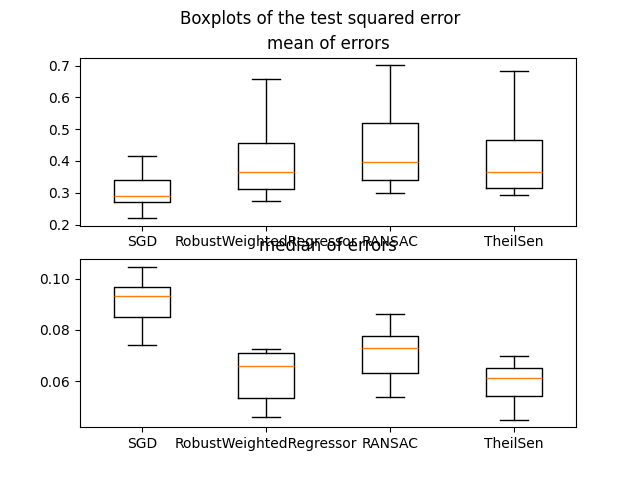
In this example we compare the RobustWeightedRegressor to other scikit-learn regressors on the real dataset california housing.

One of the main point of this example is the importance of taking into account outliers in the test dataset when dealing with real datasets.

For this example, we took a parameter so that RobustWeightedRegressor is better than RANSAC and TheilSen when talking about the mean squared error and it is better than the SGDRegressor when talking about the median squared error. Depending on what criterion one want to optimize, the parameter measuring robustness in RobustWeightedRegressor can change and this is not so straightforward when using RANSAC and TheilSenRegressor.

 Progress: 1 / 10
 Progress: 2 / 10
 Progress: 3 / 10
 Progress: 4 / 10
 Progress: 5 / 10
 Progress: 6 / 10
 Progress: 7 / 10
 Progress: 8 / 10
 Progress: 9 / 10
 Progress: 10 / 10
Text(0.5, 0.98, 'Boxplots of the test squared error')

import matplotlib.pyplot as plt
import numpy as np
from sklearn_extra.robust import RobustWeightedRegressor
from sklearn.linear_model import (
    SGDRegressor,
    TheilSenRegressor,
    RANSACRegressor,
)
from sklearn.datasets import fetch_california_housing
from sklearn.model_selection import train_test_split
from sklearn.preprocessing import RobustScaler


def quadratic_loss(est, X, y, X_test, y_test):
    est.fit(X, y)
    return (est.predict(X_test) - y_test) ** 2


X, y = fetch_california_housing(as_frame=False, return_X_y=True)
# Sub-sample for faster computation.
X = X[:1000]
y = y[:1000]

# Scale the dataset with sklearn RobustScaler (important for this algorithm)
X = RobustScaler().fit_transform(X)

# Using GridSearchCV, we do a light tuning of the parameters for SGDRegressor
# and RobustWeightedEstimator. A fine tune is possible but not necessary to
# illustrate the problem of outliers in the output.
estimators = [
    (
        "SGD",
        SGDRegressor(learning_rate="adaptive"),
    ),
    (
        "RobustWeightedRegressor",
        RobustWeightedRegressor(
            weighting="huber",
            c=0.1,
            sgd_args={
                "learning_rate": "invscaling",
            },
        ),
    ),
    ("RANSAC", RANSACRegressor()),
    ("TheilSen", TheilSenRegressor()),
]

M = 10
res = np.zeros(shape=[len(estimators), M, 2])

for f in range(M):
    print("\r Progress: %s / %s" % (f + 1, M), end="")

    rng = np.random.RandomState(f)

    # Split in a training set and a test set
    X_train, X_test, y_train, y_test = train_test_split(
        X, y, test_size=0.2, random_state=rng
    )

    for i, (name, est) in enumerate(estimators):
        cv = quadratic_loss(est, X_train, y_train, X_test, y_test)

        # It is preferable to use the median of the validation losses
        # because it is possible that some outliers are present in the
        # test set.
        # We compute both for comparison.
        res[i, f, 0] = np.mean(cv)
        res[i, f, 1] = np.median(cv)

fig, (axe1, axe2) = plt.subplots(2, 1)
names = [name for name, est in estimators]

axe1.boxplot(res[:, :, 0].T, labels=names)

axe2.boxplot(res[:, :, 1].T, labels=names)


axe1.set_title("mean of errors")
axe2.set_title("median of errors")

fig.suptitle("Boxplots of the test squared error")