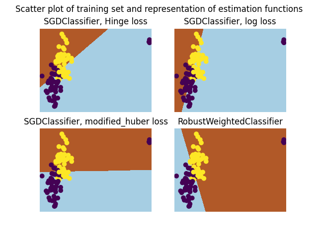
A demo of Robust Classification on Simulated corrupted dataset

In this example we compare the RobustWeightedClassifier using SGDClassifier for classification with the vanilla SGDClassifier with various losses.

Out:

/home/docs/checkouts/readthedocs.org/user_builds/scikit-learn-extra/checkouts/latest/examples/plot_robust_classification_toy.py:70: MatplotlibDeprecationWarning: shading='flat' when X and Y have the same dimensions as C is deprecated since 3.3.  Either specify the corners of the quadrilaterals with X and Y, or pass shading='auto', 'nearest' or 'gouraud', or set rcParams['pcolor.shading'].  This will become an error two minor releases later.
  ax.pcolormesh(xx, yy, Z, cmap=plt.cm.Paired)
/home/docs/checkouts/readthedocs.org/user_builds/scikit-learn-extra/checkouts/latest/examples/plot_robust_classification_toy.py:70: MatplotlibDeprecationWarning: shading='flat' when X and Y have the same dimensions as C is deprecated since 3.3.  Either specify the corners of the quadrilaterals with X and Y, or pass shading='auto', 'nearest' or 'gouraud', or set rcParams['pcolor.shading'].  This will become an error two minor releases later.
  ax.pcolormesh(xx, yy, Z, cmap=plt.cm.Paired)
/home/docs/checkouts/readthedocs.org/user_builds/scikit-learn-extra/checkouts/latest/examples/plot_robust_classification_toy.py:70: MatplotlibDeprecationWarning: shading='flat' when X and Y have the same dimensions as C is deprecated since 3.3.  Either specify the corners of the quadrilaterals with X and Y, or pass shading='auto', 'nearest' or 'gouraud', or set rcParams['pcolor.shading'].  This will become an error two minor releases later.
  ax.pcolormesh(xx, yy, Z, cmap=plt.cm.Paired)
/home/docs/checkouts/readthedocs.org/user_builds/scikit-learn-extra/checkouts/latest/examples/plot_robust_classification_toy.py:70: MatplotlibDeprecationWarning: shading='flat' when X and Y have the same dimensions as C is deprecated since 3.3.  Either specify the corners of the quadrilaterals with X and Y, or pass shading='auto', 'nearest' or 'gouraud', or set rcParams['pcolor.shading'].  This will become an error two minor releases later.
  ax.pcolormesh(xx, yy, Z, cmap=plt.cm.Paired)

import matplotlib.pyplot as plt
import numpy as np
from sklearn_extra.robust import RobustWeightedClassifier
from sklearn.linear_model import SGDClassifier
from sklearn.datasets import make_blobs
from sklearn.utils import shuffle


rng = np.random.RandomState(42)

# Sample two Gaussian blobs
X, y = make_blobs(
    n_samples=100, centers=np.array([[-1, -1], [1, 1]]), random_state=rng
)

# Change the first 3 entries to outliers
for f in range(3):
    X[f] = [20, 3] + rng.normal(size=2) * 0.1
    y[f] = 0

# Shuffle the data so that we don't know where the outlier is.
X, y = shuffle(X, y, random_state=rng)

estimators = [
    (
        "SGDClassifier, Hinge loss",
        SGDClassifier(loss="hinge", random_state=rng),
    ),
    ("SGDClassifier, log loss", SGDClassifier(loss="log", random_state=rng)),
    (
        "SGDClassifier, modified_huber loss",
        SGDClassifier(loss="modified_huber", random_state=rng),
    ),
    (
        "RobustWeightedClassifier",
        RobustWeightedClassifier(
            max_iter=100,
            weighting="mom",
            k=8,
            random_state=rng,
        ),
        # The parameter k is set larger the number of outliers
        # because here we know it. max_iter is set to 100. One may want
        # to play with the number of iteration or the optimization scheme of
        # the base_estimator to get good results.
    ),
]


# Helping function to represent estimators
def plot_classif(clf, X, y, ax):
    x_min, x_max = X[:, 0].min() - 0.5, X[:, 0].max() + 0.5
    y_min, y_max = X[:, 1].min() - 0.5, X[:, 1].max() + 0.5
    h = 0.02  # step size in the mesh
    xx, yy = np.meshgrid(
        np.arange(x_min, x_max, h), np.arange(y_min, y_max, h)
    )
    Z = clf.predict(np.c_[xx.ravel(), yy.ravel()])

    # Put the result into a color plot
    Z = Z.reshape(xx.shape)
    ax.pcolormesh(xx, yy, Z, cmap=plt.cm.Paired)
    ax.scatter(X[:, 0], X[:, 1], c=y)


fig, axes = plt.subplots(2, 2)

for i, (name, estimator) in enumerate(estimators):
    ax = axes.flat[i]
    estimator.fit(X, y)
    plot_classif(estimator, X, y, ax)
    ax.set_title(name)
    ax.axis("off")

fig.suptitle(
    "Scatter plot of training set and representation of"
    " estimation functions"
)
plt.show()