Note
Go to the end to download the full example code
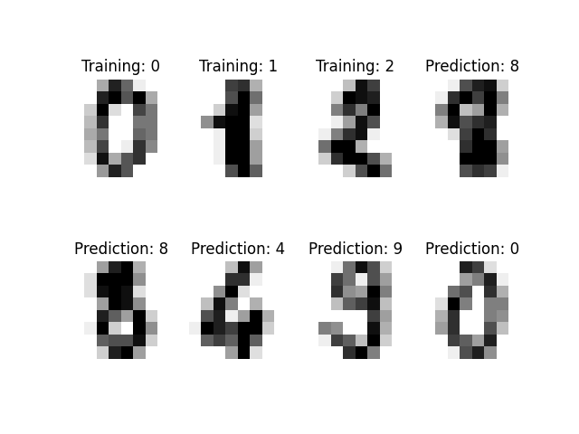
Recognizing hand-written digits using Fastfood kernel approximation
This shows how the Fastfood kernel approximation compares to a dual and primal support vector classifier. It is based on the plot_digits_classification example of scikit-learn. The idea behind Fastfood is to map the data into a feature space (approximation) and then run a linear classifier on the mapped data.
/home/docs/checkouts/readthedocs.org/user_builds/scikit-learn-extra/envs/stable/lib/python3.7/site-packages/sklearn/svm/_base.py:1208: ConvergenceWarning: Liblinear failed to converge, increase the number of iterations.
  ConvergenceWarning,
Classification report for dual classifier SVC(gamma=0.001):
              precision    recall  f1-score   support

           0       1.00      0.99      0.99        88
           1       0.99      0.97      0.98        91
           2       0.99      0.99      0.99        86
           3       0.98      0.87      0.92        91
           4       0.99      0.96      0.97        92
           5       0.95      0.97      0.96        91
           6       0.99      0.99      0.99        91
           7       0.96      0.99      0.97        89
           8       0.94      1.00      0.97        88
           9       0.93      0.98      0.95        92

    accuracy                           0.97       899
   macro avg       0.97      0.97      0.97       899
weighted avg       0.97      0.97      0.97       899


Classification report for primal linear classifier LinearSVC():
              precision    recall  f1-score   support

           0       0.95      0.94      0.95        88
           1       0.89      0.85      0.87        91
           2       0.96      0.99      0.97        86
           3       0.95      0.84      0.89        91
           4       0.97      0.93      0.95        92
           5       0.82      0.90      0.86        91
           6       0.95      0.99      0.97        91
           7       0.99      0.87      0.92        89
           8       0.85      0.85      0.85        88
           9       0.81      0.93      0.87        92

    accuracy                           0.91       899
   macro avg       0.91      0.91      0.91       899
weighted avg       0.91      0.91      0.91       899


Classification report for primal transformation classifier LinearSVC():
              precision    recall  f1-score   support

           0       0.99      0.99      0.99        88
           1       0.99      0.99      0.99        91
           2       1.00      0.98      0.99        86
           3       0.94      0.86      0.90        91
           4       0.98      0.96      0.97        92
           5       0.92      0.97      0.94        91
           6       0.99      1.00      0.99        91
           7       0.93      1.00      0.96        89
           8       0.95      0.94      0.95        88
           9       0.93      0.93      0.93        92

    accuracy                           0.96       899
   macro avg       0.96      0.96      0.96       899
weighted avg       0.96      0.96      0.96       899


Confusion matrix for dual classifier:
[[87  0  0  0  1  0  0  0  0  0]
 [ 0 88  1  0  0  0  0  0  1  1]
 [ 0  0 85  1  0  0  0  0  0  0]
 [ 0  0  0 79  0  3  0  4  5  0]
 [ 0  0  0  0 88  0  0  0  0  4]
 [ 0  0  0  0  0 88  1  0  0  2]
 [ 0  1  0  0  0  0 90  0  0  0]
 [ 0  0  0  0  0  1  0 88  0  0]
 [ 0  0  0  0  0  0  0  0 88  0]
 [ 0  0  0  1  0  1  0  0  0 90]]
Confusion matrix for primal linear classifier:
[[83  0  0  0  1  2  2  0  0  0]
 [ 2 77  1  3  0  0  0  0  6  2]
 [ 1  0 85  0  0  0  0  0  0  0]
 [ 0  0  0 76  0  6  0  1  5  3]
 [ 0  0  0  0 86  0  0  0  0  6]
 [ 0  3  1  0  0 82  2  0  0  3]
 [ 0  0  1  0  0  0 90  0  0  0]
 [ 0  0  0  0  1  6  0 77  1  4]
 [ 0  6  1  0  1  2  1  0 75  2]
 [ 1  1  0  1  0  2  0  0  1 86]]
Confusion matrix for for primal transformation classifier:
[[87  0  0  0  1  0  0  0  0  0]
 [ 0 90  0  0  1  0  0  0  0  0]
 [ 1  0 84  1  0  0  0  0  0  0]
 [ 0  0  0 78  0  5  0  4  4  0]
 [ 0  0  0  0 88  0  0  0  0  4]
 [ 0  0  0  0  0 88  1  0  0  2]
 [ 0  0  0  0  0  0 91  0  0  0]
 [ 0  0  0  0  0  0  0 89  0  0]
 [ 0  1  0  2  0  1  0  1 83  0]
 [ 0  0  0  2  0  2  0  2  0 86]]
print(__doc__)

# Author: Gael Varoquaux <gael dot varoquaux at normalesup dot org>
# Modified By: Felix Maximilian Möller
# License: Simplified BSD

# Standard scientific Python imports
import numpy as np
import pylab as pl

# Import datasets, classifiers and performance metrics
from sklearn import datasets, svm, metrics

from sklearn_extra.kernel_approximation import Fastfood

# The digits dataset
digits = datasets.load_digits()

# The data that we are interested in is made of 8x8 images of digits,
# let's have a look at the first 3 images, stored in the `images`
# attribute of the dataset. If we were working from image files, we
# could load them using pylab.imread. For these images know which
# digit they represent: it is given in the 'target' of the dataset.
for index, (image, label) in enumerate(zip(digits.images, digits.target)):
    pl.subplot(2, 4, index + 1)
    pl.axis("off")
    pl.imshow(image, cmap=pl.cm.gray_r, interpolation="nearest")
    pl.title("Training: %i" % label)
    if index > 3:
        break

# To apply an classifier on this data, we need to flatten the image, to
# turn the data in a (samples, feature) matrix:
n_samples = len(digits.images)
data = digits.images.reshape((n_samples, -1))
gamma = 0.001
sigma = np.sqrt(1 / (2 * gamma))
number_of_features_to_generate = 1000
train__idx = range(n_samples // 2)
test__idx = range(n_samples // 2, n_samples)

# map data into featurespace
rbf_transform = Fastfood(
    sigma=sigma, n_components=number_of_features_to_generate
)
data_transformed_train = rbf_transform.fit_transform(data[train__idx])
data_transformed_test = rbf_transform.transform(data[test__idx])

# Create a classifier: a support vector classifier
classifier = svm.SVC(gamma=gamma)
linear_classifier = svm.LinearSVC()
linear_classifier_transformation = svm.LinearSVC()

# We learn the digits on the first half of the digits
classifier.fit(data[train__idx], digits.target[train__idx])
linear_classifier.fit(data[train__idx], digits.target[train__idx])

# Run the linear classifier on the mapped data.
linear_classifier_transformation.fit(
    data_transformed_train, digits.target[train__idx]
)

# Now predict the value of the digit on the second half:
expected = digits.target[test__idx]
predicted = classifier.predict(data[test__idx])
predicted_linear = linear_classifier.predict(data[test__idx])
predicted_linear_transformed = linear_classifier_transformation.predict(
    data_transformed_test
)

print(
    "Classification report for dual classifier %s:\n%s\n"
    % (classifier, metrics.classification_report(expected, predicted))
)
print(
    "Classification report for primal linear classifier %s:\n%s\n"
    % (
        linear_classifier,
        metrics.classification_report(expected, predicted_linear),
    )
)
print(
    "Classification report for primal transformation classifier %s:\n%s\n"
    % (
        linear_classifier_transformation,
        metrics.classification_report(expected, predicted_linear_transformed),
    )
)

print(
    "Confusion matrix for dual classifier:\n%s"
    % metrics.confusion_matrix(expected, predicted)
)
print(
    "Confusion matrix for primal linear classifier:\n%s"
    % metrics.confusion_matrix(expected, predicted_linear)
)
print(
    "Confusion matrix for for primal transformation classifier:\n%s"
    % metrics.confusion_matrix(expected, predicted_linear_transformed)
)

for index, (image, prediction) in enumerate(
    zip(digits.images[test__idx], predicted)
):
    pl.subplot(2, 4, index + 4)
    pl.axis("off")
    pl.imshow(image, cmap=pl.cm.gray_r, interpolation="nearest")
    pl.title("Prediction: %i" % prediction)
    if index > 3:
        break

pl.show()
Total running time of the script: ( 0 minutes 1.179 seconds)